Free Shipping logo FREE SHIPPING £75+
50 years of Telonic Instruments Ltd logo CELEBRATING 50+ YEARS
Price Match logo PRICE MATCH GUARANTEE

How can I optimize the Peak scan measurements on a DSA spectrum analyser?

Posted on: December 16th, 2020 by Doug Lovell

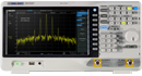
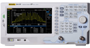
Spectrum analysers are extremely helpful tools for visualising signals in frequency space. This note will describe how to use settings to minimize error when performing peak measurements using a Rigol DSA Spectrum analyser.

Radio Frequency signals, especially continuous wave (CW) signals, have a finite frequency width.  Spectrum analysers, like the Rigol DSA series, use the 
Resolution Bandwidth Setting (RBW) to determine the bandwidth of the filter used analyse each resolution. For a fixed span, smaller RBW settings will equate to smaller frequency “steps” and finer frequency resolution measurement capabilities.  

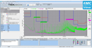
If the bandwidth of the source is less than the RBW setting of the spectrum analyser, the resultant spectrum analyser trace will have a finite width and a shape very much like a Gaussian or Bell curve as shown in Figure 1.  

In Figures 1through 4, the input is a fixed 10MHz Sine wave. The only difference is the RBW setting  on the DSA. As you can see, the width of the trace decreases as the RBW decreases. This is because the width of the RF input is less than the RBW value. We are effectively viewing the width of the RBW filter.  

It’s also important to point out that the shape of the peak of the trace also changes. It goes from a “bubbled” shape with no real “peak” to a more pointed shape. Traces with “bubbled” shapes may have peak readings that vary because there is not a singular point that is has the highest amplitude.  
     
To achieve high accuracy peak measurements, you should use the smallest RBW setting that you can. If you have varying peak values, try lowering the RBW value and retest.  
 
  
Figure 1: 10MHz input, 300kHz span, RBW = 30kHz 
  

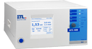
Figure 2: 10MHz input, 300kHz span, RBW = 10kHz 
 
    
Figure 3: 10MHz input, 300kHz span, RBW = 3kHz 
 
  
Figure 4: 10MHz input, 300kHz span, RBW = 1kHz

Using Excel and VBA with DSA800 spectrum Analysers

Posted on: December 16th, 2020 by Doug Lovell

Microsoft Excel and Visual Basic for Applications (VBA) is a great way for engineers who need to analyse and archive data from their instrument to access the data without deep programming skills.

With this in mind, we have created VBA examples for some of our instruments including this one for Spectrum Analyzers including the DSA800 family.

Download the example file here

Users should also install UltraSigma to make certain all the necessary drivers exist on their system. 

Download the UltraSigma install pack here

Once UltraSigma is installed, the VBA macros can be used to communicate with the instrument. We have added a few buttons to make capturing a spectrum from the instrument simple.

Here is a look at the spreadsheet:


Download further instructions for getting started using this Excel file here

NRSC AM Measurements using a DSA

Posted on: December 16th, 2020 by Doug Lovell

The Rigol DSA815 Spectrum Analyser has a built in Limit Line test that can be a convenient way to measure and compare spectral power against specific masks used for various signal types. 
One common test is NRSC Amplitude Modulation (AM) test. In this example, we are going to use the Pass/Fail mask to evaluate an AM Channel vs. limits set up by the National Radio Systems Committee (NRSC). 

Here is an excerpt from the FCC rule 73.44 

“The emissions of stations in the AM service shall be attenuated in accordance with the requirements specified in paragraph (b) of this section. Emissions shall be measured using properly operated and suitable swept-frequency RF spectrum analyser using a peak hold duration of 10 minutes, no video filtering, and a 300 Hz resolution bandwidth, except that a wider resolution bandwidth may be employed above 11.5 kHz to detect transient emissions. 
Alternatively, other specialized receivers or monitors with appropriate characteristics may be used to determine compliance with the provisions of this section, provided that any disputes over measurement accuracy are resolved in favour of measurements obtained by using a calibrated spectrum analyser adjusted as set forth above.” 

This provides the instrument settings we will use throughout this example.

1.    Set Center Frequency to match the channel you are monitoring. In this example, we are testing 1100kHz 
•    Press Freq > Center and adjust using the keypad or scroll wheel
 

2.    Set Span. In this case, we are testing AM NRSC which currently specifies 100kHz. 
•    Press Span > Span and adjust using the keypad or scroll wheel
 

3.    Set RBW and VBW.  This example requires 300Hz RBW and no video filter. 
We cannot disable VBW, but setting it larger than RBW effectively disables it.
•    Press BW/Det > RBW and adjust using the keypad or scroll wheel to 300Hz
•    While in the BW/Det menu, adjust the VBW to 3MHz. 

4.    Configure the analyser for a timed total. This test is specified for a total data collection time of 10 minutes. The easiest method to enable a timed test is to use the sweep and trigger controls of the instrument. 
•    Press Sweep > Mode > Single
•    Set Sweep Number > 600 ( at approximately 1.111s/sweep, this is a bit over 10 minutes)
 

5.    Set trace type to Max Hold
•    Press Trace > Trace Type > Max Hold

6.    Build Pass/Fail Limit line 
•    Build This can be performed manually or programmatically. See the Application Note titled “How do I create limit lines manually on the DSA815 series? or the Pass/Fail Limit builder software available for download on the DSA815 Product page located here www.rigolna.com

7.    Enable the Mask by pressing Trace/P/F > Pass/Fail > Switch On
•    Option: Pass/Fail Limit line press Trace/P/F > On > Setup
•    Option: Fail Stop Off/On to control the End Test On Failure Mode
•    Option: Beeper on Fail Off/On (P/F Menu 2/2)

8.    When ready to start the test, press Sweep/Trig > Single 
•    You can check the sweep count on the right hand side of the display
 

9.    After the test is complete, you can save a bitmap to an external USB memory. 
•    Insert USB stick into front USB port and wait for instrument to recognize the USB device.
•    If the device is not recognized, try another memory stick. USB drives with minimal files and folders will have a greater degree of success. Erase unneeded files and retry. 
•    Press the printer icon to save a BMP. 
NOTE: You can also save CSV data by pressing the Storage key.

10.    Clear traces and retest
•    Turn off mask – Press Trace/P/F > Off
•    Press Trace > Trace 1 > Type > Blank
•    Press Trace > Trace 1> Type > Max Hold
•    Press Trace/P/F > On
•    Press Start to begin test

How do I measure FM Deviation with a DSA?

Posted on: December 16th, 2020 by Doug Lovell

General purpose spectrum analysers like the Rigol DSA series can be used to test the deviation of an FM signal. 

In this example, we are going to measure the FM deviation of a 10MHz FM signal with a DSA815. This is Rigol’s 1.5GHz spectrum analyser. 
NOTE: We are starting from Factory default settings. See the User’s Guide for the instrument you are using to learn more about restoring factory defaults. 
 
1.    Set the center frequency of the analyser to the carrier frequency of the FM signal.  
 
Press FREQ > Press Center Freg >  set Center Frequency using the scroll wheel or keypad 
 
2.    Set the Span to cover the expected frequency deviation of the input signal. 
 
Press SPAN > press Span >  set using the scroll wheel or keypad 
 
3.    Set the resolution bandwidth (RBW) to provide the resolution that is required for the test.  
 
Press BW/Det > Press RBW >  set using the scroll wheel or keypad 
 
4.    Enable a second trace type as Max Hold. We will leave trace 1 (yellow) as a 
Clear Write type. This will display the input values in “real time” and trace 2 (purple) will provide a histogram of the max values achieved for all scans. 
 
Press Trace/P/F > Select Trace 2 > Set Trace Type to Max Hold 
 
5.    Let the instrument scan for a period of time long enough to build a complete envelope of the modulated signals frequency deviation.  


The DSA815 has 10 divisions on the display. The span in this example is 20kHz. So, each division is 2kHz. In this example the FM deviation is approximately 2kHz.

What is the fastest sweep time in Zero Span mode with a Spectrum Analyser?

Posted on: December 16th, 2020 by Doug Lovell

The Rigol DSA815 Spectrum analyser features a zero span mode that can be helpful in observing modulated signals. In swept mode, the detector of the analyser is sweeping across a span of frequencies at a predefined rate. The display then shows the amplitude vs. frequency of that swept scan.  

In zero span mode, the detector is fixed at a selected center frequency with a bandwidth set by the resolution bandwidth (RBW) setting. The analyser then sweeps time. This effectively puts the analyser into a mode where the X-axis represents time and the Y-axis denotes amplitude. The display is then amplitude vs. time, much like an oscilloscope.  

The DSA-815 has a minimum sweep time of 20us in Zero span mode. In the following section, we show some of the outputs of the DSA with a modulated input. 

The source waveform is a 50MHz sine wave that was burst at various rates.  The burst period is measured from the leading edge of successive bursts.  

Hopefully this can help you to gauge whether the Zero Span Mode can help you with your modulation studies.   
  

Figure 1: Burst period 5us.  
 
  
Figure 2 : 50MHz Carrier sine wave zoom.  
 
  
Figure 3: 50MHz sine wave with a burst period of 10uS as captured by an Oscilloscope.  
 
  
Figure 4: 50MHz sine wave with a burst period of 10uS.  
      
There are 10 divisions on the display, so each division is 2us. In the case of the 10us burst, you can see that the peaks are separated by 5 divisions which equals  10us. So, the programmed sourced value and the measured values match.  
If we decrease the burst period to 5us, you can see that we increase the number of “peaks” displayed on the Spectrum Analyzer and the separation between the peaks is equivalent to the burst period. 
 
  
Figure 5: 50MHz sine wave with a burst period of 10uS.  
 
  
Figure 6: 50MHz sine wave with a burst period of 5uS.

How to use UltraSigma to retrieve trace data from a DSA800

Posted on: December 16th, 2020 by Doug Lovell

1.    Download and install UltraSigma software 
 
2.    Physically connect instrument to LAN network and get IP address. You can check the IP address by pressing SYSTEM > IO SETTING > LAN 


Here the base IP address and the VISA Resource ID are highlighted 
 
3.    Open the UltraSigma software and Select LAN 
 
  
4.    From here, you can search for instruments or specify the IP address of an instrument that you would like to connect to. On closed systems (without firewalls), you can try an Auto search for Rigol Instruments that are connected to the LAN by selecting the Search button 


5.    If your Search does not produce any connection, try entering the IP address in the Manual Input area. Press Test to check the connection. 


6.    After selecting the VISA resource, UltraSigma will display the DSA800 VISA ID as shown below: 
 
  
7.    Right-Click on the resource you wish to control, and select SCPI Panel Control 
 
        
8.    SCPI panel control provides an area to send single commands and return response strings from the instrument that you are connected to.  
 
  
9.    To collect trace data from the DSA800, type the string “:TRACe:DATA? TRACe1” in the text box and press Send Command: 
 
         
10.    Now, press Read Response to bring back the data 
 
       
11.    If the data set is larger than the bytes returned, you can increase the return buffer size by changing the return byte size in the advanced tab as shown below: 
 
   
12.    Change the Bytes to be read and press OK 
 

13.    Now, press Send Command again to send “TRACe:DATA? TRACe1” and then read the response: 
 
   
14.    You can scroll down to see that the entire data set has been transferred. 
 
15.    Now, right-click on the data and Copy to Clipboard: 
 
  
16.    Open up a copy of Word or Notepad, and paste the data. 
  
      
17.    Save data as a CSV.  
 

How to Load an RSA3000 License Option

Posted on: December 16th, 2020 by Doug Lovell
Loading a License on an RSA Spectrum Analyzer is simple.

First, you receive the PDF file with the License key to install:


Enter the license Key and the Instrument serial number into the website

https://licenseen.rigol.com/CustomerService/ProductRight_EN


The verification code is the text to the right.

For the RSA instruments this generates a .LIC file that you can load onto a USB stick.

The files always have the filename equal to the Serial number, so only load one at a time to the USB stick to avoid changing the filenames or replacing the files.

Once you move the LIC file to a USB stick you can start the RSA Spectrum Analyzer and then insert the USB drive into any of the USB ports.

On the instrument hit the FILE button then use the touchscreen or mouse to navigate to the USB stick and the LIC file that you wish to load. Highlight the file so that it is in Blue and then go to the second page on the FILE menu using the down arrow. The screen should now look like this:


Once there, push the IMPORT LICENSE menu item.

This will complete the process.

At any time you can verify what is installed in an RSA instrument by pushing SYSTEM, ABOUT SYSTEM, and then selecting OPTION INFO. This popup appears:


<

Rigol USA Web Site


For Assistance in North America:

Call Us @ 877.474.4651

Email Us @ help@rigol.com

www.rigolna.com

For Assistance in Europe:

Call Us @ +49 (0)89-8941895-01

www.rigol.eu

For Assistance in China:

No.8 Ke Ling Road,

Hi-tech Development Zone,3

Suzhou,China 21516

info-intl@rigol.com

Sales: +86-512-69585066

Fax: +86-10-80720067

www.rigol.com

For Assistance in Other Countries:

info-intl@rigol.com

int.rigol.com


Warranty Terms
Activate

How to check the version of UltraSpectrum software

Posted on: December 16th, 2020 by Doug Lovell

How to check the version of UltraSpectrum software

  • Start UltraSigma software
  • Select the spectrum analyser that you wish to control by left-clicking on the instrument ID string
  • Right-click and select UltraSpectrum

  • Select Advanced Operation near the upper-right-hand-side of the window and then select About along the lower tab as shown below:

Defective UltraSpectrum display with DSA800 series

Posted on: December 16th, 2020 by Doug Lovell

If you experience a defective UltraSpectrum display while connected to a DSA800 series spectrum analyser the most likely cause is due to a UltraSpectrum software version mismatch. Software version  00.01.00.27 corrects the issue and can be downloaded from the blue Downloads tab at:

https://www.rigolna.com/products/spectrum-analyzers/dsa800/

Here is an example of the UltraSpectrum display using an incompatible version of software:

How can sweep time effect my Spectrum Measurements?

Posted on: December 16th, 2020 by Doug Lovell

Spectrum analysers can be used to observe modulated signals. But, some settings may have to be adjusted to observe the signals clearly.
In this example, we are going to show how the sweep time and selected detector type can effect the displayed data.

Source: Rigol DG4062 60MHz Dual Channel Arbitrary waveform generator.
Signal: Sine wave, linear sweep from 230KHz – 270KHz, Sweep frequency of 120Hz (~8ms period)
From the factory preset default mode, many spectrum analysers such as the Rigol DSA815-TG select an automatic sweep time which is determined by the frequency span and the RBW setting. In this example, we set the DSA to sweep from 150KHz to 600KHz at an RBW of 10KHz. The sweep rate default value for these parameters is 10ms.

In addition, the DSA815-TG collects 601 frequency “bins” per sweep. This means that the data in each bin is collected at a rate of 16us/point (10ms/601 points).
In this experiment, note that the modulation period (1/120Hz = 8ms) is much lower than the sweep rate (10ms) of the instrument.

When the sweep time is faster than the modulation, the data collected per sweep may not accurately represent the total span of the modulation. You can use the “Peak Hold” feature that will display the maximum values for successive scans and hold them on the display.

The figure below is a Peak Hold Scan for the experimental modulated signal described above. 


You can see that the sweep time is 10mS.

Also note that the Yellow scan was collected using a Peak detector and the Pink was collected using an RMS Voltage detector.
How can the Peak and RMS Voltage detectors give the same trace?
The scan rate is too fast. This results in very small data sets at each frequency bin and can cause the data collected with different detectors to appear very similar.
Now, let’s change the sweep rate and observe the differences.

Here is the same input signal with the sweep time set to 1.5s (Peak Hold Disabled/Trace Clear Write selected):


You can now see that there are some differences in the Positive Peak Data (Yellow) and the RMS Average Voltage (Pink). This includes some of the modulation peaks and a different noise floor.
Here is the same input signal with the sweep time set to 5s (Peak Hold Disabled/Trace Clear Write selected):

Now you can observe quite different traces that more accurately represent the modulated data.

Here is the same input signal with the sweep rate set to 10s (Peak Hold Disabled/Trace Clear Write selected):

Conclusions: When observing modulated or pulsed signals, you can use the Peak Hold feature to “build” a trace from successive scans.

You can also gain more visibility into the signal type by changing the detector, but keep in mind that this may require lengthing the sweep time. This will allow the instrument to collect enough data at each frequency value to make more meaningful measurements.

EMI Test System Software Getting Started Guide

Posted on: December 16th, 2020 by Doug Lovell

The Rigol EMI Test System Software is designed to make precompliance scanning with a Rigol DSA family of Spectrum Analyzer easy. 

This Note is an addendum to the Software User’s Guide. We will set up a prescan, create an amplitude correction table, set limit lines, and perform a final scan. 

Initial Setup: 

–    Download the latest version of UltraSigma and the EMI Test System Software from the Rigol website. 
–    Connect your instrument (USB, LAN, or other) and set up the physical test environment (cabling, Device-Under-Test, etc..) 
–    Start UltraSigma 
–    USB connected instruments should appear in the UltraSigma Resource tree as shown below: 


–   Right-click on the resource and select EMI Test System 
  

–    The EMI Test System will perform a screen grab of the Spectrum Analyzer and open: 


Configure Prescan Parameters 
 
–    Press Edit Scan to open the scan parameters window 
 
 
–    A Pre Scan consists of subrange elements. You can use the Pre Scan Configure window to set the overall Scan Start, Scan Stop, Range, and Detector type to use throughout the test: 
 
      
Pre Scan Configuration sets the overall test parameters used in each subrange scan. Using a Positive Peak detector will allow you to perform a faster scan and identify problem areas: 
 
In this example, we have configured the first subrange to sweep from 9kHz to 10MHz  at an RBW of 1MHz, no attenuation, and no preamplifier. 


–    Subrange Configuration sets the parameters used for each subrange step: 
 
In this example, we add a second step that goes from 10MHz to 30MHz in  at an RBW of 300kHz: 
 
  
Build successive subrange configurations using Range Start and Range Stop values and use the Add, Insert Before, After, and Delete to arrange the scan 
 
–    Press OK after you have built the Pre Scan list: 


–    Press Prescan to collect prescan data: 


After the scan is complete, you should have a graphical display of each subrange stitched together onto one graph: 


–    Now you can add amplitude correction by pressing Ampt Corr: 
 
    
–    You can select Antenna, Cable, Other, or the User tab to specify which correction table to edit.  
 
–    Enter the frequency point and corresponding  correction level. Press Add to add the correction point to the table. Repeat until the full correction table is built. 
 
–    To apply a correction table, select the type (Antenna, Cable, Other, or User) from the check boxes and press Correction: 
  
 
–    You can save the correction files for later use by pressing the Save button. 
 
You can add limit lines by pressing Peak Search to bring up the Peak Search window: 

      
–    You can add points to the limit line one-at-a-time by entering the frequency and level, then press add. Here, we have built a limit line comprise of four sections. You can also save the limit lines to recall them later by pressing Save: 
 
  
–    Use History to recall saved limit lines 
 
–    Press OK to apply the limit lines 
 
 
–    All of the peaks that have failed the limit test are shown at the bottom of the display: 
 
      
–    You can find specific peaks by clicking on the Peak number: 
 
  
–    You can also change the Vertical and Horizontal Scales by selecting the scales from the Y Unit and X Axis drop down boxes: 
  
 
–    You can print out a report of scanned data by pressing the Report button and filling in any information that you need. 

 
–    If you have found areas that fail the limit lines, you can save time by performing another prescan. This time, set the start and stop frequencies to encompass the failing peak(s). 
 
–    In this more focused scan, you may also want to use a Quasi Peak detector and FCC RBW settings (if your analyser is equipped with those options.

DSA800 Prefix: How to more easily save filenames

Posted on: December 16th, 2020 by Doug Lovell

The latest revision of firmware (DSA815 00.01.12) has the ability to save a prefix for use with file saves. This can make data entry a bit easier.

–    Press SYSTEM > Down arrow to page 2 > Select Name Prefix

–    Select EDIT PREFIX and use the keypad to enter the text you want to start the files with

–    Press OK

–    Here, we have saved TEST as the prefix

–    Set PREFIX SWITCH to ON when you want to use the prefix

NOTE: You can leave the text box in the numeric control (“1” shown in lower corner) when you close the text entry window. It will appear in the same state next time you save a file. You can simply press 1,2,3..etc.. to increment the file.