 FREE SHIPPING £75+
 CELEBRATING 50+ YEARS
 PRICE MATCH GUARANTEE
When using a differential probe with a real time spectrum analyser you will be using the instrument in General Purpose mode and then you will need to create a reference signal that can be referenced when using the differential probe to compare the two signals, then once the reference has been created next you will then use the build in trace math feature to compare the reference signal that was created to the currently measured signal, this will create the actual differential signal.
First create a reference trace – to do this you will need to connect the Vout+ to the positive end of the differential probe and then the negative end of the differential probe to ground. Once these have been connected set the spectrum analysers frequency span to equal the differential probe’s span, for the RP1100D it is 9kHz to 100MHz and for the RP1050D it is 9kHz to 50MHz. With the span set now turn on the spectrum analysers reference amplitude in the amplitude menu to 0 dBm, this may need to be changed depending on the signal.
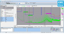
With the spectrum analyser configured set the differential probe to X100 and then configure the amplifier so that it is producing a single tone at 9 kHz with an amplitude set to the amplifiers maximum output. Then enter the trace/p/f menu on the spectrum analyser, select the 2nd trace and then set the trace type to max hold and then begin to sweep across the frequency range with the amplifier. Use as small of steps as possible between the frequency points as this will make the reference more accurate. Now that you have created a reference signal freeze this signal, to do this now change the trace type to freeze in the trace/p/f menu. You will then have a reference signal similar to the one pictured below.
(Reference signal is pictured in blue)
Next use the trace math function to create the actual measured differential signal – Next leave Vout+ connected to the positive probe and then connect the negative probe to Vout-. Then use the spectrum analyser’s trace math feature to the compare the reference trace on trace 2 to the real time differential trace on trace 1. For this test I have terminated Vout+ and Vout- to a 50-ohm load, after the probe connection. This will create the green signal shown below.
(Note that I do not have Vout+ or Vout- currently turn on in the image. Reference trace in blue, math comparison and differential signal in green.)
In order to confirm the results, I have set both Vout+ and Vout- to output a 50 MHz sine wave with 0dBm of amplitude and they are shown below to have the same amplitude resulting in a math signal with an amplitude of 0 dBm. Shown below.
(Reference trace in blue, math comparison and differential signal in green.)
To take amplitude measurements use the marker function – To measure the amplitude use the marker function with the marker trace set to math. Below shows the reference signal with Vout+ with an amplitude of -10dBm and Vout- with an amplitude of 0 dBm and shown below is the difference in amplitude. Due to how it is calculated the amplitude is half of the difference which in terms of dB is roughly -3.5 dBm.
(Reference trace in blue, math comparison and differential signal in green.)


How to take differential measurements on a RSA5000
S1210 Changing the Workspace path
When the S1210 application is started up a default Workspace path and demo file is created. In the example below the demo Workspace file has been created in C:/Users/ruby/AppData/Local:
The S1210 application now shows the associated demo tests that be selected and you can connect to the spectrum analyser by clicking on Device:
A different Workspace path can be selected if desired. In the example below the path has been set to C:/Temp/S1210:
No tests have been created so there are now no tests listed in the example below. And, without a test you will not be able to connect with the spectrum analyser when you click on Device:
To create a new test select File and then New. In the example below test_0 has been created. Now that a test exists you can select Device to connect to the spectrum analyser.
Measuring Cable Loss with a Spectrum Analyser
A spectrum analyser with a tracking generator can be a useful piece of test gear. This application note covers making a simple loss measurement on a coaxial cable with BNC connectors.
Required:
– Two N-type to BNC Adapters. Select adapters that convert N-type (in/out connectors on most spectrum analyzers) to the cable type you are testing. Also note that higher quality connectors (Silver plated, Beryllium Copper pins, etc..) equal better longevity and repeatability.
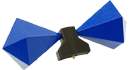
Figure 1: N-type to BNC adapter
– A short reference cable with terminations that match your adapters and cableunder-test.
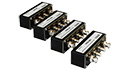
– An adapter to go between the reference cable and the cable-under-test. This experiment will use a BNC “barrel connector”. Note that higher quality connectors (Silver plated, Beryllium Copper pins, etc..) equal better longevity and repeatability.
Figure 2: BNC barrel adapter
– Alternately, you can use two adapters a short cable as a reference assembly to normalize the display before making cable measurements. This removes the need to have the cable-to-cable adapter.
– Spectrum analyser with Tracking Generator (TG)
Steps:
1) Turn on Spec An and attach adapters to the tracking generator (TG) output and RF Input.
2) Connect the reference cable to the TG out and RF In.
Figure 3: Measuring reference cable
3) Adjust Span of scan for frequency range of interest.
4) Adjust TG output amplitude and spectrum analyser display to view the entire trace.
5) Enable TG.
Figure 4: Reference cable insertion loss before normalization.
6) Normalize the reference insertion loss. This mathematically subtracts a reference signal (stored automatically) from the input signal.
– With the Rigol DSA815 Press TG > NORMALIZE > STOR REF and then Enable
Normalize
Figure 5: Reference cable insertion loss after normalization.
7) Disconnect the reference cable from the RF input.
8) Place cable-to-cable adapter (BNC barrel or other) and connect to the cable to test.9) Connect the cable-under-test to test to RF input and enable the TG.
Figure 6: Cable-under-test connected.
The screen displays the cable-under-test losses plus the error of the cable-to-cable adapter.
Figure 7: Cable-under-test loss.
UltraSpectrum License Activation instructions
Ultra Spectrum is a software package that enables remote control and data collection from Rigol DSA spectrum analyzers.
It is available for trial.
After the trial period has expired, you can purchase an activation license by contacting your local Rigol sales office.
Here are instructions for activating your license:
- Download and install UltraSigma software (see Ultra Sigma instructions for more information)
- Download and install Ultra Spectrum
- Power on and connect your DSA via USB or Ethernet to the controlling PC
- Run UltraSigma. This should bring up a screen as below.. with your DSA information.
- Right-click on the resource, and select UltraSpectrum
6. You will get a prompt telling how many days left on your trial. Click Activate
7. Enter the license code (Reg Code) and click OK
NOTE: License codes are linked to the instrument serial number.
Working with correction factors
Some applications require adjusting the displayed amplitude to accurately account for losses in cables, gain in amplifiers/antennas, and other circuit elements.
This note presents the steps to create, save, and recall correction factors on a DSA800 Series manually and programmatically.
Create a Correction Factor (manually):
1. Press AMP > Down Arrow > Corrections
2. Select Antenna, Cable, Other, or User. These labels name temporary (volatile) storage of the correction value that you are entering.
3. Press Edit and use the key pad to enter the correction point and amplitude that cover the frequency range of interest. You can enter multiple points to create a correction profile for a particular antenna, cable, other, or user setting.
4. Press the back arrow to go back one menu.
5. Enable the Correction Table by pressing Corr Table ON. Verify the corrections are the proper values entered above.
Figure 1: Correction Table enabled. In this example, there are two points set to show a -40dB correction from 0Hz to 1GHz.
Store a Correction Factor:
1. Once you have created the correction profile for the element (antenna, cable, etc..) of choice, Press Storage
HINTS: Change file type to CORRECTIONS to see correction files.
• Make sure you have used the Dir (directory) selection to choose either Local (:D) drive or the Mobile Disk (:E) USB drive.
• After you have selected a drive, change Browser to File to select and open file location or choose to overwrite an existing file.
• Put an indication of correction type in the file name. “A1” for antenna 1, “C1” for cabling setup 1, etc… This will make recalling the file easier in the future.
Figure 2: Storage screen for the DSA. Note the Local drive is selected (Left hand side) as is the first corrections file shown. The filter type is set to Corrections.
Correction files terminate in *.cbl.
2. Press Save and enter the name using the keypad.
• When you press a number, “3” for example, the letters under the number will appear. “3” has d, e, and f. Pressing the 3 again will advance the highlighted cursor from d to e. Press again, and it will go from e to f.
• You can select capitalize letters by pressing the “1” key
• Press “+/-” to toggle between Chinese, English Alphabet, and Numbers.
3. Press OK to save the file.
NOTE: Correction values are stored under the label used to create them. For example, if you create an antenna correction factor and store it, it will be located under antenna when you go to recall it.
Create a Correction factor (programmatically):
You can also programmatically construct and activate correction files by using the following steps:
1. Build the correction table by sending the command:
:CORR:CSET<n>:DATA<freq>, <rel_ampl>,{,<freq>, <rel_ampl>}
Where <n> = Internal memory location (0-9) for the file
<freq> = Frequency in Hz
<rel_ampl> = Correction value
2. To enable the correction table, send:
:CORR:CSET<n> ON
3. To save the correction table, send:
:MMEM:STOR:CORR <file_type>,<file_name>
Where <file_type> = ANT|CABL|OTH|USER
4. Here is an example of creating a correction factor of -10dB from 1Hz to 1GHz and storing the file on a DSA815.
The commands were sent using UltraSigma SCPI Panel Control.
You can enable the table manually by pressing AMPT > Down Arrow to page 2 > Corrections and selecting the proper correction file from memory Recall a Correction factor:
1. Press Storage
NOTE: Insert USB drive if the correction factors were stored externally.
1. Select File Type filter to Corrections to show only corrections (*.cbl) files
2. Select the appropriate browser directory (DIR) to locate the file location
3. Change the browser to FILE and select the correction file of interest
NOTE: The File Name will be highlighted when it is selected!
If the file name is not highlighted, you will need to select it using Browser > File.
4. Press the down arrow to go to the Storage Menu page 2/3.
5. Press Recall to recall the file.
6. To confirm the correction, enable the corrections and corrections table
• Press AMPT > Down Arrow > Corrections
• Select the correction factor (antenna, cable, other, user)
• Enable correction factor by pressing Correction > On
• Enable correction table by pressing Corr Table > On
NOTE: Correction values are stored under the label used to create them. For example, if you create an antenna correction factor and store it, it will be located under antenna when you go to recall it.
How to measure a filter using a RIGOL Spectrum Analyser
This document provides step-by-step instructions on using the Rigol DSA-800 series of Spectrum Analysers to measure the characteristics of an RF Bandpass filter.
NOTE: The DSA must have a Tracking Generator to effectively perform the following test.
Normalize the trace (Optional)
Many elements in an RF signal path can have nonlinear characteristics. In many cases, these nonlinear effects on your base measurements can be minimized by normalizing the instrument.
1. Connect tracking generator output to RF input using the same cabling that you will be using to test your device. Any element, like an adapter, used during normalization should also be used during device measurement as any changes to the RF signal path could effect the accuracy of the measurement.
2. Enable the tracking generator by pressing the TG button > TG On
3. Store the reference trace by pressing the TG button > Normalize > Stor Ref
4. Enable normalization by pressing the TG button > Normalize > Normalize On
Measure the filter
1. Connect the tracking generator output to the filter input using the appropriate cabling and connectors.
2. Connect the filter output to the instrument RF input.
3. Set the tracking generator amplitude by pressing the TG button and the TG Amplitude. You can use the keypad or wheel to enter the correct value.
NOTE: If your instrument is equipped with a Preamplifier, you can enable it to lower the displayed noise floor by pressing the following sequence:
Amplitude button > Down Arrow > RF Preamp On
4. Enable the Tracking generator by pressing the TG button > RF Source ON You can see the small bump in the figure below.
Figure 1: Before Auto.
5. You can use the Auto button to center and zoom on the waveform. You can also use the Freq and Span buttons to manually manipulate the displayed data.
Figure 2: After Auto.
6. You can now enable the Marker function to measure the bandwidth and attenuation or passband characteristics of the filter.
7. Press Marker Fctn > N dB BW and set the function to the amplitude of interest. In this example, we are measuring the 3dB Bandwidth of our filter.
How to measure an RF Amplifier using a RIGOL Spectrum Analyser
This document provides step-by-step instructions on using the Rigol DSA-800 series of Spectrum Analysers to measure the characteristics of an RF Amplifier.
In addition to the DSA-800 Spectrum Analyser, you will need an RF Source, cabling, and adapters.
Measure the amplifier
1. Connect the RF generator output to the RF input of the instrument using the appropriate cabling and connectors.
NOTE: If your instrument is equipped with a Preamplifier, you can enable it to lower the displayed noise floor by pressing the following sequence:
Press AMP button > Down Arrow > RF Preamp On
Figure 1: Preamplifier off
Figure 2: Preamplifier on
2. You can use the Auto button to center and zoom on the waveform. You can also use the Freq and Span buttons to manually manipulate the displayed data.
• Another option to center the waveform is to press Freq button > Peak → CF. This will automatically align the center of the display with the peak of the trace.
3. Freeze the unamplified trace by pressing Trace > Trace Type > Freeze. You can use the Marker button to create a marker. This can be used to find the peak frequency and amplitude of the displayed waveform.
4. Disable the RF Generator output.
5. Disconnect RF generator from the instrument RF Input and connect it to the Amplifier input.
6. Connect the Amplifier output to the instrument RF Input.
7. Enable the RF generator.
8. Enable a second trace to visualize the amplified signal by pressing the Trace button > Select Trace 2.
9. Set the trace type to Clear/Write by pressing Trace > Type > Clear/Write.
10.You can use the Auto button or manually center the trace using the Freq, Span, and Amp buttons.
11.Readjust the amplitude scale by pressing Amp > Auto
12.You can enable an additional marker for the new trace by pressing Marker > Select the marker you would like to use
13. Now, select the trace you want to mark by pressing Marker > Marker Trace
> select trace of interest
• Be sure Normal is selected to enable the marker
14.You can also enable a marker table by pressing Marker > Down Arrow > Mkr Table ON. This allows a convenient way to compare markers and values between traces.
15. Alternately, you can use the Trace Math function to create a Trace difference on the screen.
16. Enable Trace Math by pressing Trace > Trace Math
17. Set Function to A-B
18. Set A = T1
19. Set B = T2
20. Set Operate > On
21.Set Amplitude by pressing AMPL > Auto
NOTE: New trace appears. This represents Trace 1 – Trace 2.
22. Set Marker to Math Trace by pressing Marker > select Marker 3
23.Set Marker Trace to Math by pressing Marker > Marker Trace > Math
• You can then move the marker to the smoothest portion of Trace 3.
DSA-815 License Activation
The Rigol DSA-815 Spectrum Analyser has a number of optional features that can be activated by obtaining an activation license.
Currently, the advanced measurement kit (DSA8-AMK), VSWR (DSA8-VSWR), and EMI Toolkit (DSA8-EMI) are available.
First, obtain the license key from your local Rigol representative.
The code is a 24 character code of alphanumerics.
Here is a sample:
XXX-XXX-XXX-XXX
- Power on the instrument
2. Press System > Down Arrow
3. Press Install
4. A textbox will appear
5. Use the EDIT Keypad on the front panel to enter the alphanumeric code shown on the license.
NOTE: The “1” key will capitalize the letters (A/a).. The “+/-” key will toggle between Chinese (Shown as CN in the textbox), English(EN), and Number (1). Press the numeric character that contains the letter of interest. Multiple presses of the number key will scroll through the available characters. Press ENTER key to accept the letter.
6) Press the OK key after you have entered all of the characters. The instrument should indicate that the license option has been activated.
Can I use the tracking generator on a DSA as a fixed RF source?
Many spectrum analysers, like the Rigol DSA800 series, have tracking generator options available. The tracking generator is an RF source that follows the frequency sweep settings of the spectrum analyser.
For example, if you configure a spectrum analyser to sweep from 100 to 200MHz, and enable the tracking generator, the output of the generator would output a swept sine from 100 to 200MHz at the set amplitude. This sweeping function is useful when characterizing the frequency response of filters and amplifiers.
Figure 1: Response of a filter to a swept RF input using a tracking generator on a spectrum analyser.
You can also use a tracking generator as a fixed frequency RF source by simply using the spectrum analyser in Zero Span Mode.
In this note, we are going to configure a DSA815-TG in Zero Span mode to source a 50MHz Sine wave.
1. Set the center frequency to 50MHz by pressing FREQ > Center Frequency and set the value to 50MHz using the keypad or scroll wheel
2. Set the span to zero by pressing SPAN > select ZERO SPAN
3. Now, configure the tracking generator output by pressing TG > set the amplitude using TG LEVEL
4. Connect the RF output (TG output) of the spectrum analyser to the device under test
5. Enable the tracking generator output by pressing TG > ON
Here is a scope capture of the 50MHz output of the TG:
DSA Ethernet connectivity troubleshooting
Communicating over LAN to the DSA series is straightforward. Here are some things to try if you are having difficulty:
1. Make sure Ethernet cable is connected properly and that the switch/hubs in the network configuration are operating properly.
o The green LED on the back of the DSA should display a solid illumination when the connection is made.
o The yellow LED on the back of the DSA should blink when data is sent and received.
2. The DSA defaults to communicate over USB. To configure the instrument for Ethernet, follow these steps:
o Press System > I/O Setting > Remote I/O and toggle to LAN
• Press System to Exit the menu
3. Find LAN configuration and make sure it matches your instrument settings
• Press System > I/O Setting > LAN
• Record the IP Address, Subnet Mask, and Gateway
• Open a web browser (Chrome, Internet Explorer, etc..) and type the IP address into the address bar at the top.
• If everything is configured correctly, the DSA’s webpage will load
How to enable the log frequency scale of the DSA815
Starting at firmware revision 00.01.12, the DSA815 spectrum analyser can display the frequency scale in Log mode.
Press SPAN and set X Scale to Log
How do I save a user setup with a DSA800?
To save a setup:
1) Insert USB stick into the USB port on the front panel
NOTE: The format of the USB stick must be FAT32
2) Press STORAGE > Set BROWSER to DIR. You can press the button next to the Browser label to toggle the selection.
3) Use the scroll wheel to select Mobile Disk (E:)
4) Change File Type to Setup and press the back arrow to get back to the storage screen
5) Press Save, use the keypad to write a filename (I use numbers, they are faster), and press OK
Product Categories
AC Power Supplies / Frequency ConvertersDC Power Supplies
DC Electronic Loads
Test & Measurement
Safety Testers
EMC
Soldering Irons / Test Tools
Manufacturers
Rental
Service & Support
AboutContact
Newsletter
Service Returns Form
Returns Policy
Terms and Conditions
Privacy Policy
Shipping & Delivery
My account