Automating a test can dramatically increase the productivity, throughput, and accuracy of a process. Automating a setup involves connecting a computer to the test instrumentation using a standard communications bus like USB or LAN and then utilizing code entered via a software layer (like LabVIEW, .NET, Python, etc..) to sequence the specific instrument commands and process data.

This process normally goes quite smoothly, but if there are problems, there are some basic troubleshooting steps that can help get your test up-and-running quickly.

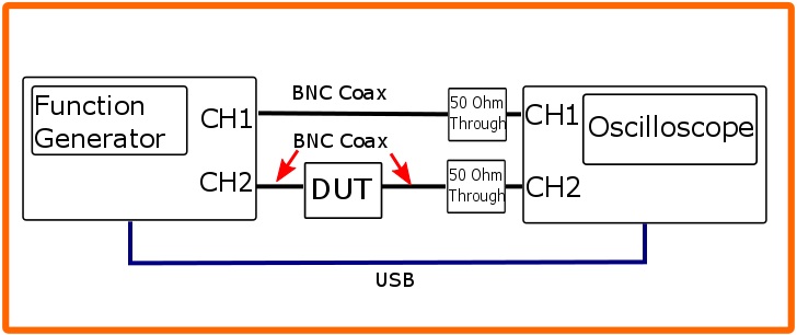
In this note, we are going to show how to use NI-MAX to test the communications connection between an instrument and a remote computer using both a USB and a LAN connection to ensure that they are working properly. Once the connection is verified, you can begin to work on the control software.

National Instruments Measurement and Automation Explorer (NI-MAX) is a free communications tool provided with NI’s VISA library.

You can learn more here: https://digital.ni.com/public.nsf/allkb/71544521BDE34FFB86256FCF005F4FB6

USB Connections

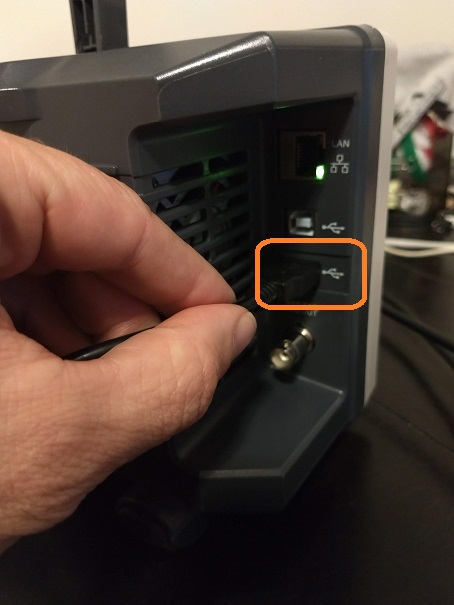
1. Power on and connect the instrument via USB cable to the computer. On a computer running Windows, the first time you connect the USB from an instrument should open a dialog box or show a notification of a new device being connected.

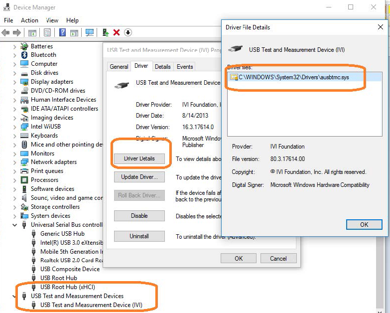
You can check the status of the USB connections by opening Device Manager located in the Control Panel menu of most Windows Operating systems and expanding the driver information as shown below in this Windows 10 example:

This indicates that the operating system recognizes the connected instrument as a test instrument.

If the device manager reports the USB connection as some other type of device (printer, camera, unknown, etc.), there is likely a problem linking the proper driver (ausbtmc.sys) to the instrument. One possible solution to this is to disable the driver, disconnect the USB cable, verify that ausbtmc.sys exists, and then reconnect the USB cable.

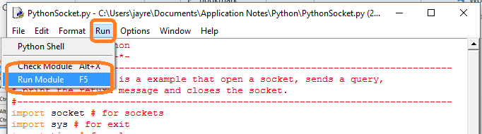
2. Run NI-MAX by left-clicking on the icon on the desktop or finding it via the start menu

3. This will open the main window, as shown below:

4. Expand the “Devices and Interfaces” menu. You should see the instruments attached via USB with a brief description as shown for an SDS2000X oscilloscope below:

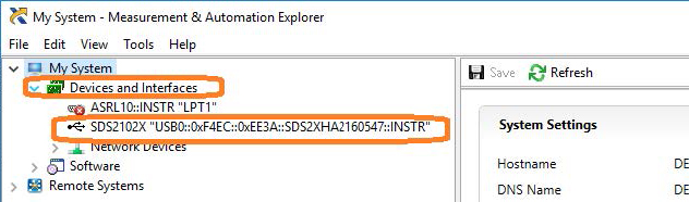
This indicates that a software application (NI-MAX) has correctly identified a test and measurement device (the oscilloscope) over the USB connection.

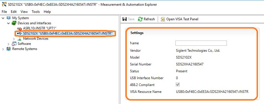
5. By left-clicking on the instrument, you can see additional information about it:

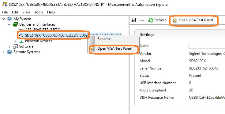
6. To further test the connection, right-click on the instrument and select Open VISA Test Panel or select it from the side bar:

The VISA Test Panel window shows some helpful information, including the instrument manufacturer, model, serial number, and the USB identifier (VISA Address) along the top.

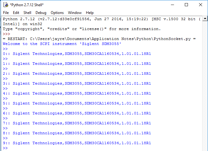
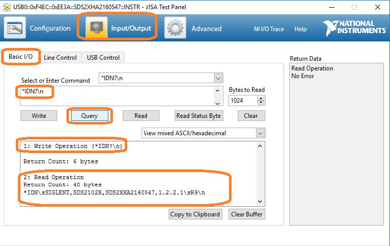
7. Another useful item in the VISA Test Panel is the Input/Output function. This mode allows you to send specific instrument commands and receive instrument responses.

This is especially helpful when you are planning a specific test sequence, the effect of delays/timing, or troubleshooting a command. You can send each
command one-at-a-time and check the performance of the instrument.

Select Input/Output > Basic I/O > and Enter the command in the text window:

– *IDN? is a common identification string query (question or information request) that returns the information from the connected instrument
– /n is a termination character that represents a new line. This is the standard termination character for SIGLENT instrumentation.
– Write will send the command to the instrument
– Read will pull data from the instrument
– Query will perform a read and then a write command to request and return data from the instrument

USB Checklist

– Is the USB port configured properly on the instrument? Some instruments feature USB ports that can be configured as TMC (Test and Measurement) or Printer communication ports. The USB port should be set to USBTMC or similar for remote control.
– Try a direct connection to the controlling computer. USB hubs or long connections may cause issues.
– Try a different USB cable. Connectors can go bad or prove to be faulty.
– Try a different USB port on the computer.
– On machines running Windows, check the Device Manager. Test instrumentation should appear as USB Test and Measurement Device (IVI) and use the AUSBTMC.SYS driver

Lan Connections

1. Power on and connect the instrument via LAN cable to a LAN network connected to the computer you wish to use.

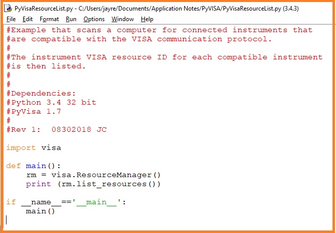
You can check the status of the LAN connection by using a software tool like NMAP: https://nmap.org/

NMAP allows you to scan networks and identify IP addresses.

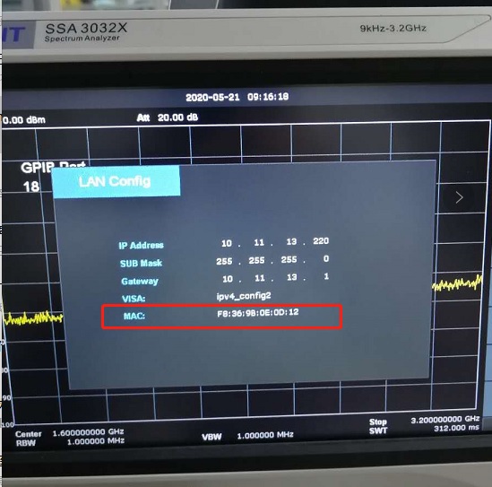
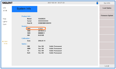
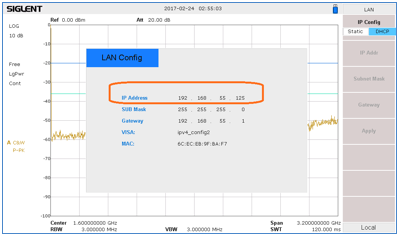
First, identify the LAN connection for the instrument. This is typically located in the System menu under IO or LAN settings.

Here is the IO information for an SDS2000X oscilloscope:

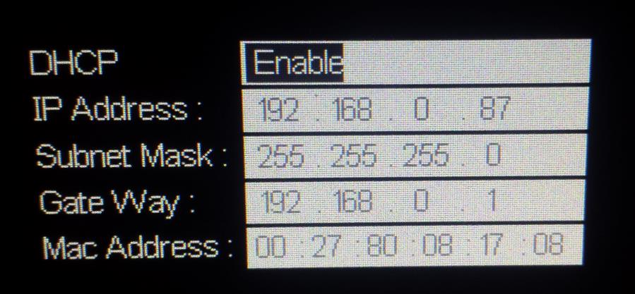
DHCP Enabled will automatically configure the instrument connection settings and apply a valid IP address. With DHCP enabled, the IP address may change over time. It is recommended to check the instrument IP address and then confirm that it is visible on the network using NMAP:

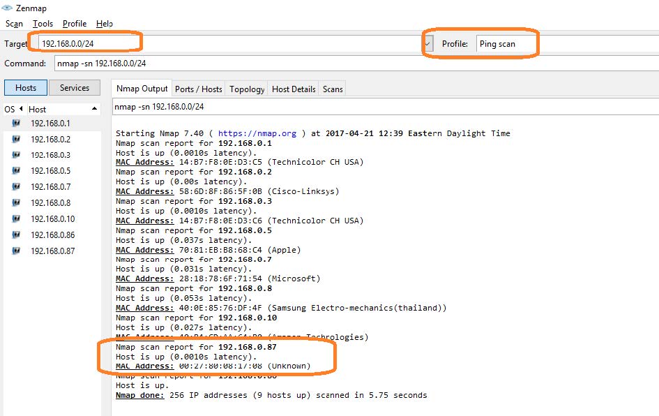
Here, we are performing a Ping (short scan to identify what IP addresses are being used) over the range of IP addresses that may match the instrument.

This can be performed by setting the target using the “/24” extension. This scans 24 bits For example, 192.168.10.0/24 would scan the 256 hosts between
192.168.10.0 and 192.168.10.255

Here is more information from NMAP:
https://nmap.org/book/man-target-specification.html

For example, to ping all IP addresses that start with 192.168.0., set the target as follows:

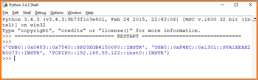
Note the IP address and MAC address that identify your instrument.

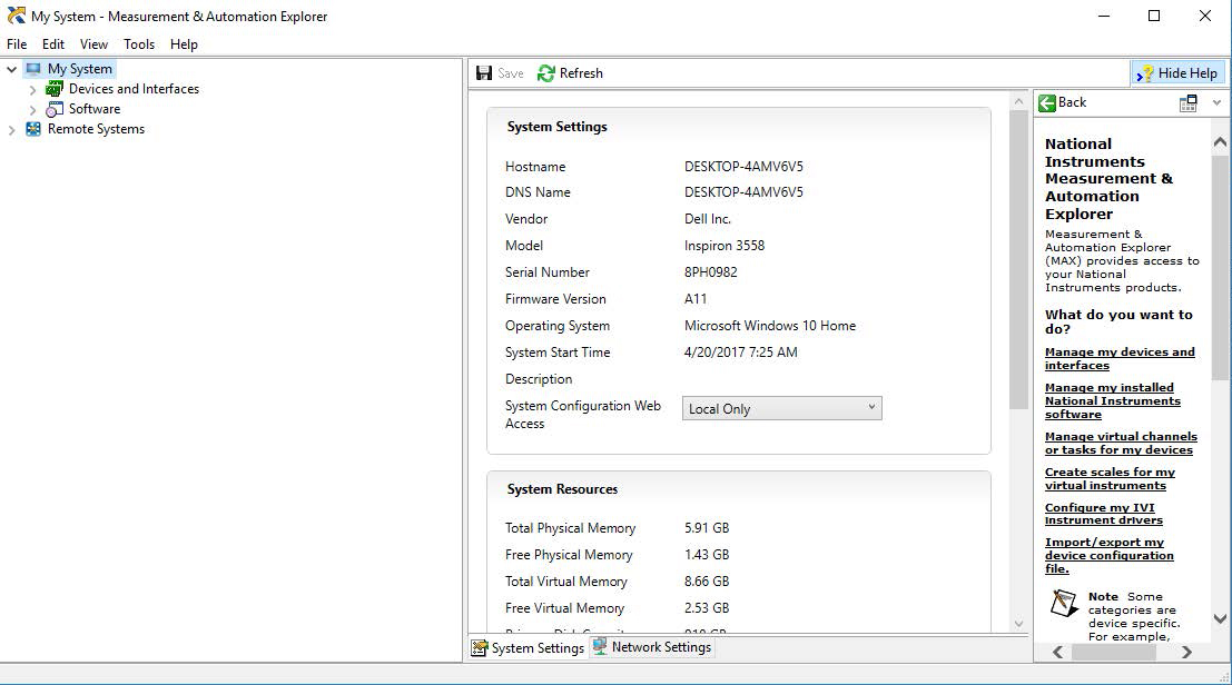
2. Run NI-MAX by left-clicking on the icon on the desktop or finding it via the start menu

This will open the main window, as shown below:

3. Unlike USB, there is not an easy way to identify all of the instruments connected via LAN.

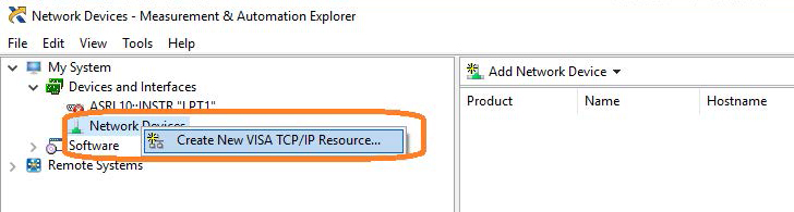
In many cases, you will have to manually add the LAN instrumentation. Recall from Step 2, our instrument IP address is 192.168.0.87

Right-click on Network Devices, and select Create New VISA TCP/IP Resource:

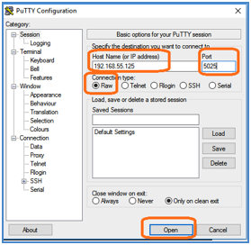
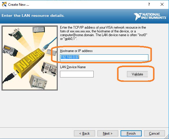
4. Select Manual Entry of LAN:

5. Enter the IP address and press Validate

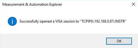
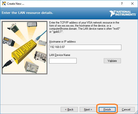
6. After successfully creating a TCP/IP connection, select finish

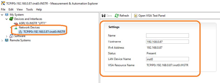
7. After the system updates it’s configuration, the instrument will appear in the Network Devices menu:

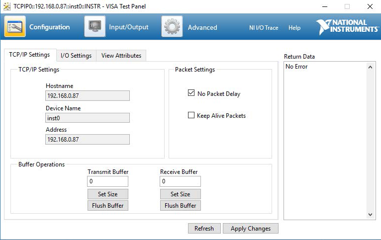
8. To further test the connection, right-click on the instrument and select Open VISA Test Panel or select it from the side bar:

The VISA Test Panel window shows some helpful information, including the TCP/IP identifier (VISA Address) along the top.

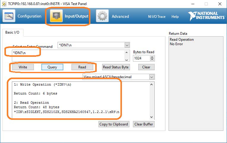
9. Another useful item in the VISA Test Panel is the Input/Output function. This mode allows you to send specific instrument commands and receive instrument responses.

This is especially helpful when you are planning a specific test sequence, the effect of delays/timing, or troubleshooting a command. You can send each command one-at-a-time and check the performance of the instrument.

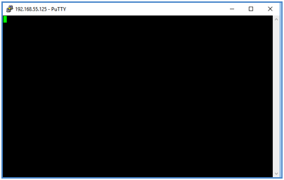
Select Input/Output > Basic I/O > and Enter the command in the text window:

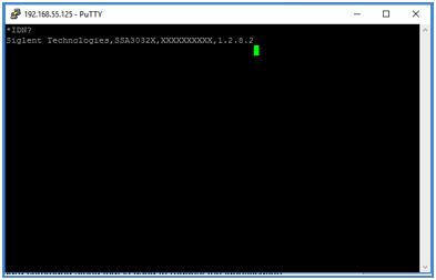
– *IDN? is a common identification string query (question or information request) that returns the information from the connected instrument
– /n is a termination character that represents a new line. This is the standard termination character for SIGLENT instrumentation.
– Write will send the command to the instrument
– Read will pull data from the instrument
– Query will perform a read and then a write command to request and return data from the instrument

For more information, check SiglentAmerica.com, or contact your local Siglent office.

Like many modern oscilloscopes, the SIGLENT SDS series feature FFT math functions that calculate frequency information from the acquired voltage vs. time data. FFT stands for Fast Fourier Transform, and is a common method for determining the frequency content of a time-varying signal. Converting time domain data to the frequency domain makes measuring characteristics like phase noise and harmonics much easier. Oscilloscopes don’t have the dynamic range or sensitivity of a true spectrum analyzer, but these new designs can provide a fine level of detail that may be just enough for your application.

FFTs are commonly used on high frequencies, but they can also be used on signals with fairly low frequencies.

In this note, I am going to show the FFT performance of two series of our scopes by sourcing a 10 mHz (100 s period), 10 Vpp sine wave using a SIGLENT SDG805 Function Generator into Channel 1.

For those interested, here are the specs for the SDG805

SDS1000X/SDS2000X Series:

The SDS1000X and 2000X series feature an FFT function that uses up to 16 kpts of timebase data to calculate the frequency data and a timebase maximum of 50 s/div.

Here are the FFT results with the available window settings for a 10 mHz sinewave –

The scope can show a split timebase and FFT view:

For the rest, I will use the exclusive FFT view.

Rectangle

Blackman

Hanning

Hamming

Flat Top

SDS1000X-E Series:

The SDS1000X-E series feature a new math co-processor that increases the maximum data depth of the FFT function to 1 Mpts. They also feature a timebase maximum of 100 s/div. These increases allow the X-E to have much finer timebase detail and to acquire useful data for even lower frequencies than many scopes on the market.

Here are the FFT results with the available window settings for a 10 mHz sinewave –

The scope can show a split timebase and FFT view:

For the rest, I will use the exclusive FFT view.

Rectangle

Blackman

Hanning

Hamming

Flat Top

The SDS series of oscilloscopes all feature remote programming and data collection capabilities. They can be integrated easily into many automated test environments to ease the setup and data acquisition during testing.

One of our helpful customers developed a nice programming example designed to set up and retrieve data from a SIGLENT SDS1202X-E Oscilloscope using Kotlin, a free open source coding environment (more on Kotlin here).

The code utilizes a LAN connection and open sockets.

Thanks to Chris Welty for the code!

Here is a text file of the example:

SDSDataRetrievalKotlinExample

/**
* License: 3-Clause BSD
*
* Copyright 2018 Chris Welty
*
* Redistribution and use in source and binary forms, with or without modification, are permitted provided that the following conditions are met:
*
* 1. Redistributions of source code must retain the above copyright notice, this list of conditions and the following disclaimer.
*
* 2. Redistributions in binary form must reproduce the above copyright notice, this list of conditions and the following disclaimer in the documentation and/or other materials provided with the distribution.
*
* 3. Neither the name of the copyright holder nor the names of its contributors may be used to endorse or promote products derived from this software without specific prior written permission.
*
* THIS SOFTWARE IS PROVIDED BY THE COPYRIGHT HOLDERS AND CONTRIBUTORS “AS IS” AND ANY EXPRESS OR IMPLIED WARRANTIES, INCLUDING,
* BUT NOT LIMITED TO, THE IMPLIED WARRANTIES OF MERCHANTABILITY AND FITNESS FOR A PARTICULAR PURPOSE ARE DISCLAIMED. IN NO
* EVENT SHALL THE COPYRIGHT HOLDER OR CONTRIBUTORS BE LIABLE FOR ANY DIRECT, INDIRECT, INCIDENTAL, SPECIAL, EXEMPLARY, OR
* CONSEQUENTIAL DAMAGES (INCLUDING, BUT NOT LIMITED TO, PROCUREMENT OF SUBSTITUTE GOODS OR SERVICES; LOSS OF USE, DATA, OR
* PROFITS; OR BUSINESS INTERRUPTION) HOWEVER CAUSED AND ON ANY THEORY OF LIABILITY, WHETHER IN CONTRACT, STRICT LIABILITY,
* OR TORT (INCLUDING NEGLIGENCE OR OTHERWISE) ARISING IN ANY WAY OUT OF THE USE OF THIS SOFTWARE, EVEN IF ADVISED OF THE
* POSSIBILITY OF SUCH DAMAGE.
*/

package scope

import java.io.BufferedWriter
import java.io.OutputStreamWriter
import java.io.Serializable
import java.net.Socket

/**
* Contains a single waveform downloaded from a Siglent 1202X-E
*/
class Waveform(val vDiv: Double, val vOffset: Double, val tDiv: Double, val tOffset: Double, val data: ByteArray) : Serializable {

val xs: DoubleArray
get() = DoubleArray(data.size, { i -> i * tDiv * 14 / data.size + tOffset – tDiv * 7 })

val ys: DoubleArray
get() = DoubleArray(data.size, { i -> data[i] * vDiv / 25 – vOffset })

companion object {
/**
* Download the waveform displayed on the scope’s screen
*/
fun download(): Waveform {
Socket(“192.168.1.222”, 5025).use { socket ->

println(“connected to ” + socket.inetAddress)
val output = BufferedWriter(OutputStreamWriter(socket.getOutputStream(), Charsets.US_ASCII))

// since the socket can return binary data, we can’t use an InputStreamReader to
// translate the bytes to characters. We’ll have to do it ourselves.
// SCPI generally uses US ASCII, shouldn’t be too hard.
val input = socket.getInputStream()

/**
* Read from the scope until \n is encountered.
* The bytes are translated to characters numerically (so US_ASCII).
*/
fun readLine(): String {
val sb = StringBuilder()
while (true) {
val c = input.read()
when (c) {
-1, ‘\n’.toInt() -> return sb.toString()
else -> sb.append(c.toChar())
}
}
}

/**
* Read a number of bytes from the scope.
*
* The bytes are not translated into characters.
*/
fun readBytes(n: Int): ByteArray {
val result = ByteArray(n)
var i = 0
while (i < n) {
i += input.read(result, i, n – i)
}
return result
}

fun writeLine(string: String) {
output.write(string)
output.write(“\n”)
output.flush()
}

/**
* Read a numerical response from the scope.
*
* The scope returns responses like “C1:VDIV 1.00E+00V”.
* This function extracts the “1.00E+00″, converts it to a double, and returns it.
*/
fun readNumber() = readLine().split(” “)[1].dropLast(1).toDouble()

writeLine(“*IDN?”)
println(readLine())

// reset the scope response format to its default so readNumber() works
writeLine(“CHDR SHORT”)

writeLine(“C1:VDIV?”)
val vDiv = readNumber()

writeLine(“C1:OFST?”)
val vOffset = readNumber()

writeLine(“TDIV?”)
val tDiv = readNumber()

writeLine(“TRDL?”)
val tOffset = readNumber()

// request all points for the waveform
writeLine(“WFSU SP,0,NP,0,F,0”)
writeLine(“C1:WF? DAT2”)

// parse waveform response
val header = String(readBytes(21))
println(“header is $header”)
val length = header.substring(13, 21).toInt()
println(“length is $length”)
val data = readBytes(length)
readBytes(2) // 2 garbage bytes at end

println(“V/div = $vDiv; offset = $vOffset; t/div = $tDiv; tOffset = $tOffset”)

return Waveform(vDiv, vOffset, tDiv, tOffset, data)
}
}
}
}

Many instruments include the ability to be controlled via a remote connection to a computer using an Ethernet connection. In many cases, these instruments require a special software library that can help establish and maintain the communications link between the instrument and controlling computer. This can be annoying for a few reasons… the software library is likely to occupy a large amount of space on the controlling computer and is also required on any computer that is being used to control the instrument. In a remote networking application where multiple user’s may want access to a test instrument, this can cause support and installation headaches.

Luckily, there are a few solutions that can help. In this application note, we are going to discuss using open socket communication techniques using an open source communication tool called PuTTY with a SIGLENT SSA3032X spectrum analyzer.

What are open sockets and why use them?

Within the context of Ethernet/LAN connections, sockets are like mailboxes. If you want to deliver information to a specific place, you need to be sure that your information is delivered to the correct address.

In the context of test instrumentation, an open socket is a fixed address (or port number) on the Ethernet/LAN bus that is dedicated to process remote commands.

Open sockets allow remote computers to simply use existing raw Ethernet connections for communications without having to add additional libraries (VISA or similar) that require additional storage space and processing overhead.

Programs that utilize sockets for LAN communication tend to take up less memory and operate more quickly.

PuTTY

PuTTY is an open source software tool that provides a number of simple communication links (RAW, Telnet, SSSH, Serial, and others). It is available for free and there are a number of versions available for popular operating systems.

You can download as well as learn more here: https://www.putty.org/

In this example, we are using PuTTY to verify the raw LAN connection is working properly. It is quite a simple program that does not allow for very complex operation (sequences, converting data sets/strings, etc..). If you require more complex functionality, software platforms like Python, .NET, C#, LabVIEW, etc.. can be used to control the instrument using a similar open socket connection.

Configuration

In this test, we are using the most current revision of the SIGLENT SSA3032X Spectrum Analyzer firmware (Revision 01.02.08.02) which enables open socket communication.

This example also uses PuTTY version 0.67:

Steps

1. Install PuTTY for the OS you intend to use

2. Make sure your instrument and firmware revision can use open sockets

The SSA3032X revision 01.02.08.02 enables open socket communication.

To find the revision, press the System button > Sys Info.

Figure 1 below shows a sample system information screen from a SIGLENT SSA3000X analyzer:

Figure 1: Sample system information page from an SSA3000X.

Check the product page and firmware release notes for more information.

3. Connect the instrument to the local area using an Ethernet cable

4. Find the IP address for the instrument. This is typically located in the System Information menu. On the SIGLENT SSA3032X, press the System button on the front panel > Interface > LAN.

Figure 2 below shows a sample LAN setup page from a SIGLENT SSA3000X:

Figure 2: Sample LAN information page from an SSA3000X.

5. Open PuTTY

6. Select Raw as connection type

7. Enter the IP address in the Host Name field

8. Enter the port number. This should be provided in the users or programming guide for the instrument.

The SIGLENT SSA3000X uses port 5025.

Figure 3 below shows the PuTTY configuration for this example:

Figure 3: Example PuTTY configuration.

9. Press Open. This will open a terminal window as shown in below:

10. Using the computer keypad, enter *IDN? and press the Enter key on the keyboard to send the command.

This is the standard command string that is used to request the identification string from the instrument. As shown below, the instrument responds with the manufacture, product ID, Serial Number, and firmware revision.

Conclusion

PuTTY is an easy way to verify an operational LAN connection to instrumentation that can use open sockets.

In AM schemes, the modulation index refers to the amplitude ratio of the modulating signal to the carrier signal. With the help of Fast-Fourier-Transforms (FFT), the modulation index can be obtained by measuring the sideband amplitude and the carrier amplitude. In this application note, we are going to show a convenient method of using the new Peaks/Markers function (Available on the 4 channel SIGLENT X-E scopes with firmware revisions > 6.1.31).

1. Basic Principle

Amplitude modulation uses a signal (typically a sine wave in the audio frequency range from 10 Hz to 20 kHz) to control the amplitude of a higher frequency signal called the carrier.

A carrier with amplitude modulation can be represented as

Where:

V(t)              The Amplitude Modulated Signal

Uc                Amplitude of the Carrier Signal

m                 Modulation Index

a(t)               Normalized Modulation Signal

fc                 Carrier Frequency

Sinusoidal (commonly referred to as a “sine” wave) modulation is the most commonly used modulation waveform type. If we are using a sine wave, the modulating signal can be expressed as

According to the formulas (1) and (2), we can get

Mathematically represents the carrier waveform.

 and represent the positive, or upper, and negative, or lower, sidebands of the modulated signal.

The amplitude of both sidebands are 

If we set the amplitude of sideband is Us,

In logarithmic case, if the difference between the sideband amplitude and the carrier amplitude is X,

Then the amplitude modulation index can be represented as

Figure  1

Here, we can see that it is easy to measure the difference between the sideband amplitude and the carrier amplitude, or X. We can then calculate the modulation index very easily.

2. Measurement Setup and Result

2.1 Equipment

Oscilloscope: Siglent SDS1204X-E with firmware version higher than 6.1.31.

Signal Source: Siglent SDG2122X

Cable: 50 ohm BNC

2.2 Instrument Configuration

In this section, we will show how to configure the instruments in order to make the measurement. For complete instructions on the FFT mode, please refer to the oscilloscope user manual and the quick start guide.

The oscilloscope is connected to the output of the signal source as shown in Figure 2.

Figure 2 Set Up for the Measurement

The signal source settings are as follows:

• Mod On
• Mod Type: AM modulation
• Carrier frequency: 1 MHz
• Carrier amplitude: 500 mVpp
• Modulation frequency: 10 kHz, and the modulation index is 80%.

According to the output of the signal source, set the center frequency of the FFT plot to 1 MHz and set the horizontal scale to 5 kHz to provide a clear view of the output.

To reduce random errors, the FFT is set to average mode and the average number of times is 100. On the choice of window function, we choose flat-roofed window to obtain the optimized amplitude accuracy.

Starting with firmware revision 6.1.31, the FFT function of Siglent X-E oscilloscopes include a Peaks/Markers function and users can set the number of FFT points separately. The more points the FFT has, the better the frequency resolution of the plot will have. Note that increasing the number of points will increase the time of computation of the FFT, which will reduce the refresh speed accordingly. FFTs up to 1 Mpts at most are available on the X-E series, so we can set the storage depth to 1.4 Mpts. In this application, there is no need for a high sampling rate, since that will lead to a large delta frequency. Set the timebase to 2ms.

According to the input signal, we can deduce that a frame waveform has 28 k-cycles and we will use the first 20 k-cycles to do the FFT operations. For decent resolution, there should be at least five sample points in a cycle, so the minimum number of FFT points should be at least 100 kpts. 128 kpts is suitable, since under the premise of satisfying the measurement conditions, we can get the results faster.

The new version also supports Peaks/Marker, it can quickly identify and label peaks. We choose Peaks to make the measurement.

Figure 3 Configuration Screens

The configuration process is as follows:

First, set timebase to 2ms and enter the ACQUIRE menu, set Mem Depth to 1.4M. Second enter the MATH menu, set Operator to FFT, enter the CONFIG menu, setMaximum points to 128k, set Window to Flattop, set Display to Exclusive then go to the next page, set Mode to Average, set Times to 100. Third enter the VERTICALmenu, set Unit to dBVrms, then enter HORIZONTAL menu, set Center to 1MHz, set Hz/div to 5 kHz. Last, enter the FFT TOOLS menu and set Type to Peaks, turn on theShow Table switch to show the peaks list and turn on the Show Frequency switch to show the frequency of peaks, set Sort By to Frequency.

2.3 Result

After configuration is done, enter SEARCH menu, adjust Threshold to show several peaks for easy reading from the table then press Reset. After the average number increasing to 100, the FFT result as shown in Figure 4.

Figure 4 FFT Peaks Result

The carrier amplitude is -14.9dBV, the sideband amplitude is -22.8dBV. So the difference between the sideband amplitude and the carrier amplitude is -7.9dB.

According to the previous introduction, the results of the modulation index are shown in the table 1.

Table 1 Measurement Result

3. Summary

The Siglent oscilloscope with newly released Peaks/Markers software, supports peak and harmonic searching which provides a convenient method of spectrum analysis.