 FREE SHIPPING £75+
 CELEBRATING 50+ YEARS
 PRICE MATCH GUARANTEE


How to Extract FFT Data from the Rigol DHO914S Using Python
If you’re using the Rigol DHO914S oscilloscope and want to perform FFT analysis beyond the scope’s built-in display, you’re in luck. This guide will show you how to:
✅ Export waveform data from the DHO914S
✅ Apply a Hanning window
✅ Compute and plot the FFT magnitude spectrum
✅ Add interactive or automatic peak markers
✅ Optionally export the results to CSV
🧾 Step 1: Export the CSV File from the Oscilloscope
On your Rigol DHO914S:
- Capture a waveform on Channel 1 (CH1).
- Press
Storage>File Type> Select CSV. - Save the data to a USB stick or via network.
- Transfer it to your PC.
You’ll get a .csv file that looks like this:
python-replCopyEditCH1V, t0 =-1.000000e-02, tInc = 2.000000e-06
-0.786533,,,
0.386800,,,
...
Step 2: Load and Process the Data in Python
Install required libraries if you haven’t already:
bashCopyEditpip install numpy pandas matplotlib scipy
Now use the following script:
pythonCopyEditimport numpy as np
import pandas as pd
import matplotlib.pyplot as plt
from scipy.signal import find_peaks

# --- Load CSV from Rigol DHO914S ---
filename = "RigolDS0.csv"  # Replace with your filename
df = pd.read_csv(filename)
voltage = df['CH1V'].dropna().to_numpy()
N = len(voltage)

# --- Sampling Information (from file header) ---
t_inc = 2e-6  # 2 µs time interval
fs = 1 / t_inc  # 500 kHz sample rate

# --- Apply Hanning Window ---
window = np.hanning(N)
windowed_signal = voltage * window

# --- Perform FFT ---
X = np.fft.fft(windowed_signal)
freqs = np.fft.fftfreq(N, d=t_inc)
half_N = N // 2
freqs = freqs[:half_N]
magnitude = (2 / N) * np.abs(X[:half_N])  # Normalized magnitude

# --- Automatically Detect Peaks ---
peak_indices, _ = find_peaks(magnitude, height=0.1)  # Adjust threshold
peak_freqs = freqs[peak_indices]
peak_amps = magnitude[peak_indices]

# --- Plot FFT Spectrum with Peaks ---
plt.figure(figsize=(10, 5))
plt.plot(freqs, magnitude, label="FFT Magnitude")
plt.plot(peak_freqs, peak_amps, 'ro', label="Detected Peaks")
for f, a in zip(peak_freqs, peak_amps):
    plt.annotate(f"{f:.1f} Hz", xy=(f, a), xytext=(f, a + 0.05),
                 ha='center', fontsize=8)
plt.title("FFT Spectrum with Peak Detection (Hanning Window)")
plt.xlabel("Frequency (Hz)")
plt.ylabel("Amplitude")
plt.grid(True)
plt.legend()
plt.tight_layout()
plt.show()

# --- Print Peak Info ---
print("Detected Peaks:")
for i in range(len(peak_freqs)):
    print(f"Peak {i+1}: Frequency = {peak_freqs[i]:.2f} Hz, Amplitude = {peak_amps[i]:.4f}")
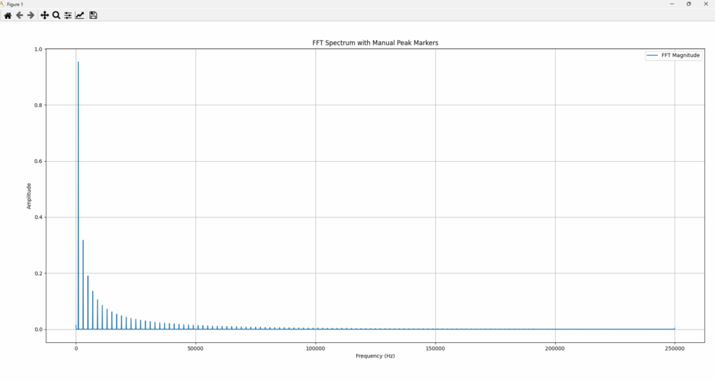
Optional: Click to Manually Mark Peaks
If you’d rather click directly on the FFT plot to inspect peaks manually:
pythonCopyEditplt.figure(figsize=(10, 5))
plt.plot(freqs, magnitude)
plt.title("Click to Mark Peaks (Press Enter When Done)")
plt.xlabel("Frequency (Hz)")
plt.ylabel("Amplitude")
plt.grid(True)
plt.tight_layout()
plt.show(block=False)

print("Click on peaks to mark them (press Enter when done)...")
clicks = plt.ginput(n=-1, timeout=0)

for i, (fx, _) in enumerate(clicks):
    idx = np.argmin(np.abs(freqs - fx))
    print(f"Marker {i+1}: Frequency = {freqs[idx]:.2f} Hz, Amplitude = {magnitude[idx]:.4f}")
Optional: Save FFT Spectrum to CSV
You can export the FFT data for use in Excel or other tools:
pythonCopyEditfft_df = pd.DataFrame({
    'Frequency (Hz)': freqs,
    'Amplitude': magnitude
})
fft_df.to_csv("fft_output.csv", index=False)
Summary
Using Python, you can go far beyond what the Rigol DHO914S shows on screen:
- Perform FFT on high-resolution waveforms
- Apply windowing functions like Hanning
- Detect or interactively mark signal peaks
- Export the data for further analysis or reporting